SQL Databases — PostgreSQL, MySQL & MSSQL
The SQL family of the Databases module covers your relational engines — PostgreSQL, MySQL, and MSSQL (SQL Server). They share one consistent investigation flow built around the questions relational operators ask most: which query is slow, what are connections waiting on, and is the engine itself under pressure?
Open Databases in the sidebar and stay on the SQL tab.
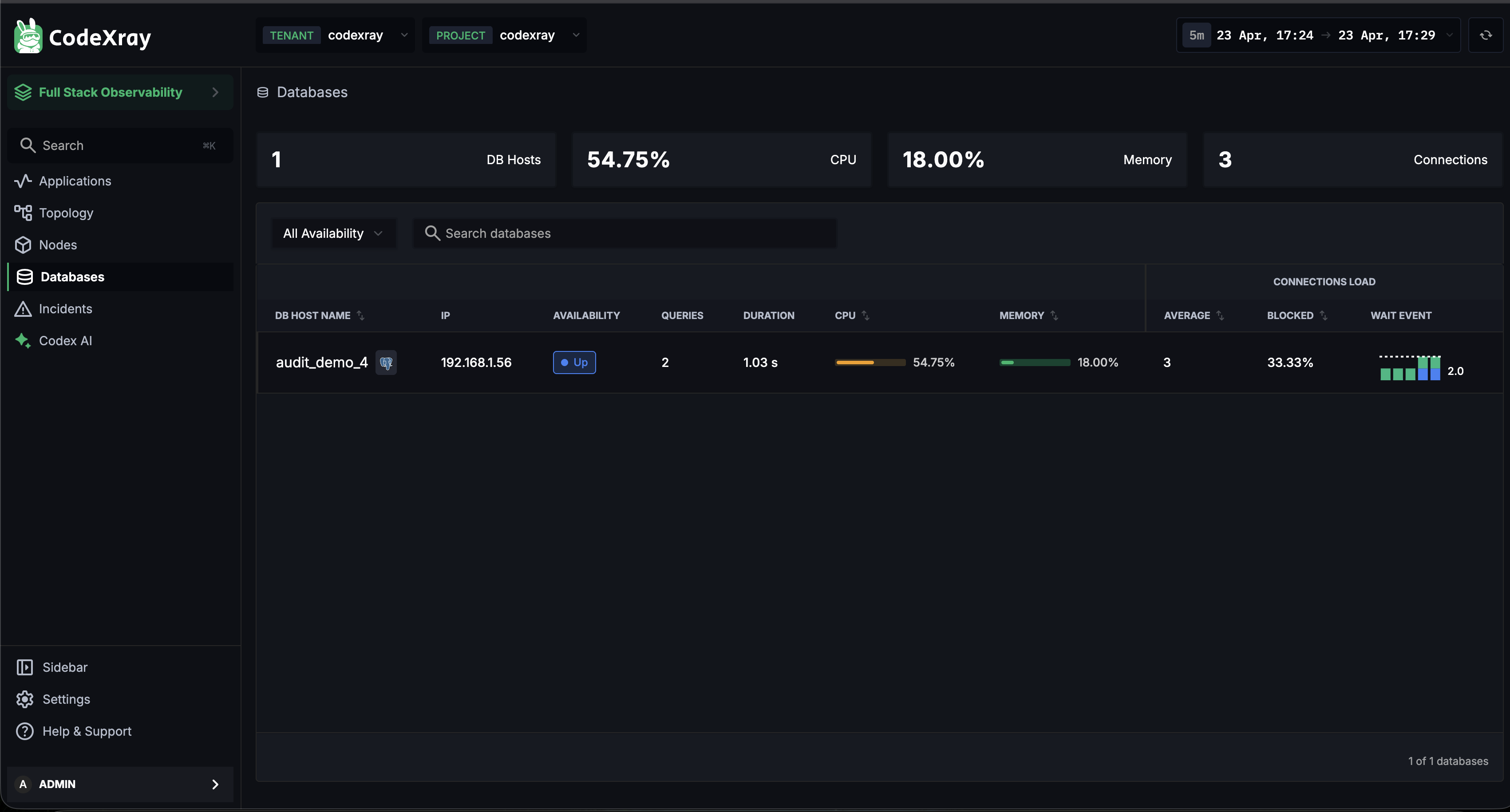
The SQL fleet list
The top of the SQL tab rolls up your entire relational fleet into four KPIs:
| KPI | What it tells you |
|---|---|
| DB Hosts | Total relational databases being monitored |
| CPU | Highest CPU pressure across the fleet |
| Memory | Highest memory pressure across the fleet |
| Connections | Aggregate active connection count |
Below the KPIs, a searchable, filterable table lists every database with its live health signals:
| Column | What it shows |
|---|---|
| DB HOST NAME | The database instance name, with an engine icon (PostgreSQL / MySQL / MSSQL) |
| IP | Host IP address |
| AVAILABILITY | Up / Down live status badge |
| QUERIES | Recent query activity |
| DURATION | Average query duration |
| CPU | CPU utilisation, with an inline bar |
| MEMORY | Memory utilisation, with an inline bar |
| CONNECTIONS LOAD — AVERAGE | Current active connection count |
| CONNECTIONS LOAD — BLOCKED | Percentage of connections waiting on a lock |
| CONNECTIONS LOAD — WAIT EVENT | A mini distribution of connection states (CPU / Lock / IO) |
Use the Availability filter and the Search databases box to scope the list when you have many instances. Click any row to open its detail view.
PostgreSQL, MySQL, and MSSQL each carry their own icon in the DB HOST NAME column, so a mixed relational fleet stays readable at a glance.
Database detail — three focused tabs
Click into any SQL database and you land on a detail page with three tabs — Top Queries, Metrics, and Active Connections. Each answers a different investigation question.
Top Queries
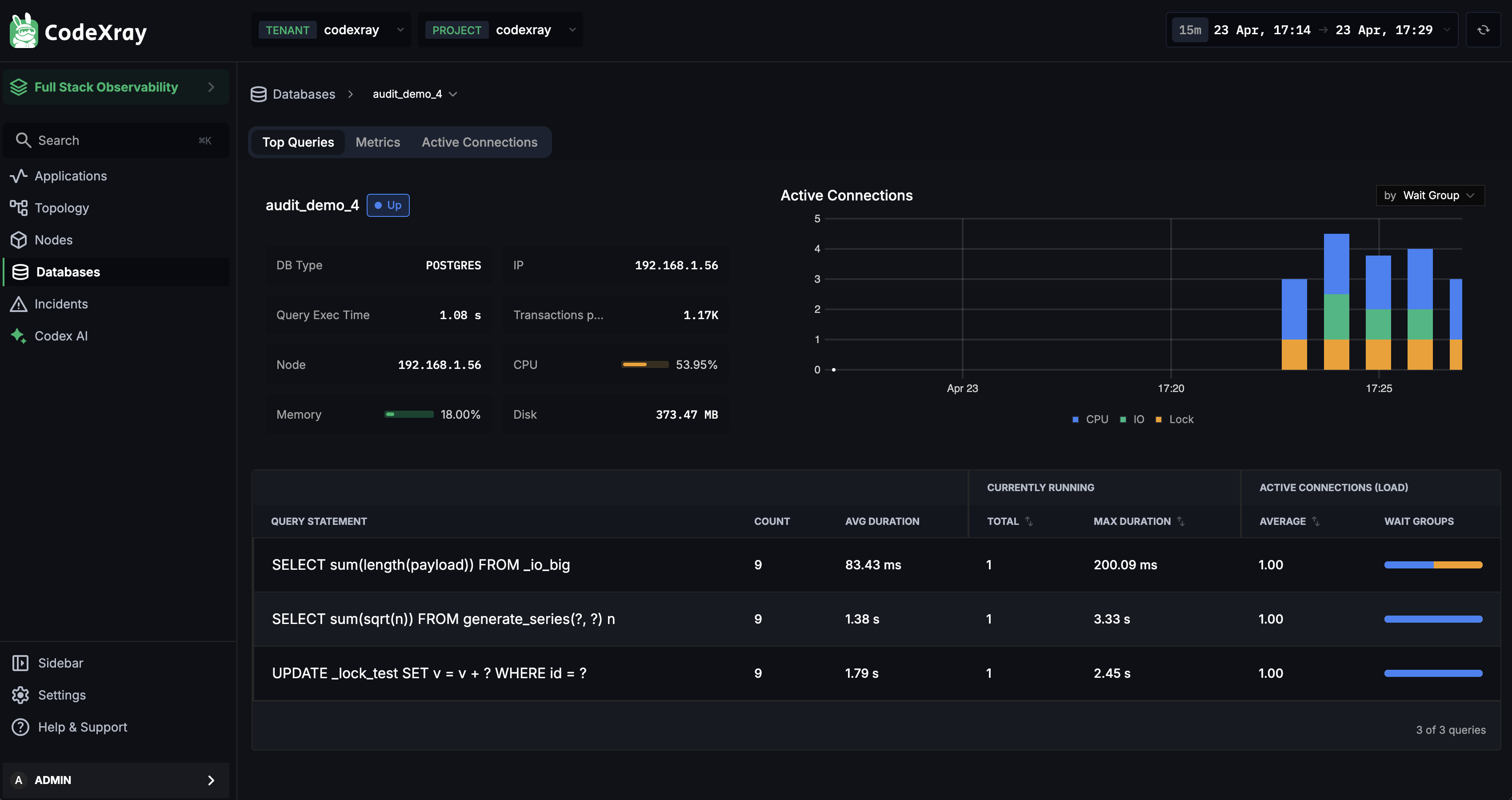
The Top Queries tab is where most performance investigations start. It surfaces the queries the engine itself has identified as significant — backed by the engine's own query statistics rather than sampling.
Database metadata strip (left) — at a glance:
- DB Type — POSTGRES / MYSQL / MSSQL
- IP and Node — where the database is running
- Query Exec Time — current average execution time
- Transactions per min — transaction throughput
- CPU / Memory — live resource usage
- Disk — disk footprint
Active Connections chart (right) — a live stacked chart of active connections grouped by Wait Group (CPU / Lock / IO). It tells you at a glance what the database is busy doing right now.
Query table (bottom) — a ranked list of queries:
| Column | What to use it for |
|---|---|
| QUERY STATEMENT | Query fingerprint — parameterised values collapsed, so variants group together |
| COUNT | How many times the query ran in the window |
| AVG DURATION | Mean execution time |
| CURRENTLY RUNNING — TOTAL | How many executions of this query are in flight right now |
| CURRENTLY RUNNING — MAX DURATION | Longest currently-running execution |
| ACTIVE CONNECTIONS LOAD — AVERAGE | Average number of connections this query is holding |
| ACTIVE CONNECTIONS LOAD — WAIT GROUPS | Which wait groups this query's connections are in |
Use Top Queries when a database is slow and you need to know which query is the cause, when capacity-planning around the queries that dominate load, or when evaluating a schema or index change.
Metrics
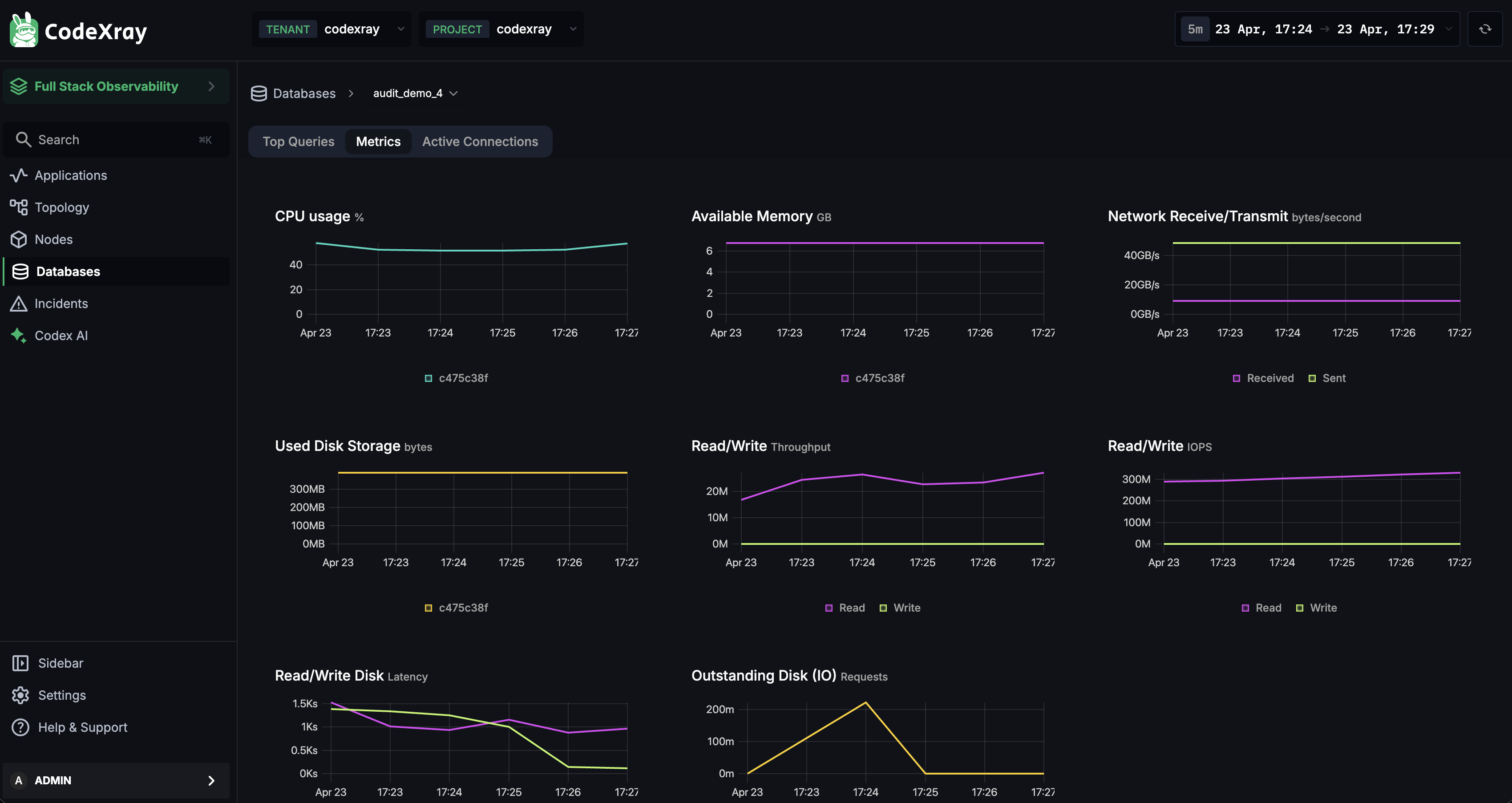
The Metrics tab is the engine's vital signs — a grid of time-series charts covering everything that matters when a database is struggling:
| Chart | What it tells you |
|---|---|
| CPU usage | How hard the database is working |
| Available memory | Free RAM — low values mean disk pressure is coming |
| Network receive / transmit | Traffic in and out — separates app-heavy from replication-heavy load |
| Used disk storage | Storage growth as a trend, not just a point-in-time number |
| Read / write throughput | Bytes read and written per second |
| Read / write IOPS | Operations per second — saturates before throughput does on SSDs |
| Read / write disk latency | How long each I/O takes — the single best indicator of I/O contention |
| Outstanding disk I/O requests | Queue depth — sustained high values mean I/O can't keep up |
Use Metrics to tell application-level slowness from engine-level saturation, when tuning the database, or when sizing hardware for an upcoming scale event.
Active Connections
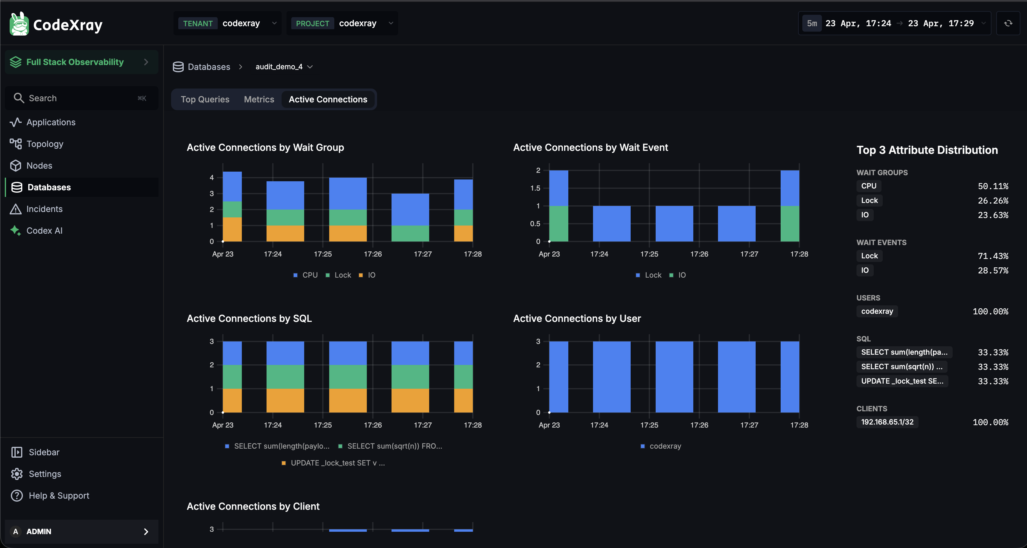
The Active Connections tab is a live, multi-dimensional breakdown of what your database's connections are actually doing right now. Five charts slice connections by different axes:
| Chart | Answers |
|---|---|
| By Wait Group | Where is time going? — CPU / Lock / IO |
| By Wait Event | What specifically is blocking? — the exact engine-reported wait |
| By SQL | Which queries are holding connections? |
| By User | Which database user is most active? |
| By Client | Which client IP / host is driving load? |
Top 3 Attribute Distribution (right panel) — a compact rollup of each dimension, with sections for WAIT GROUPS, WAIT EVENTS, USERS, SQL, and CLIENTS. It reads like a one-line summary of the engine's state — "50% of connections are in CPU wait, 26% on Lock, 24% on IO" — and makes a great screenshot to share during an incident.
Use Active Connections when you suspect a connection leak or pool exhaustion, when queries are piling up on a lock and you need the holder, or when an unexpected client IP is driving load.
PostgreSQL query plans
PostgreSQL goes one step further: from the Top Queries table you can open any query's execution plan directly in CodeXray — no psql session, no manual EXPLAIN. Click a query row to open the Query Explanation panel.
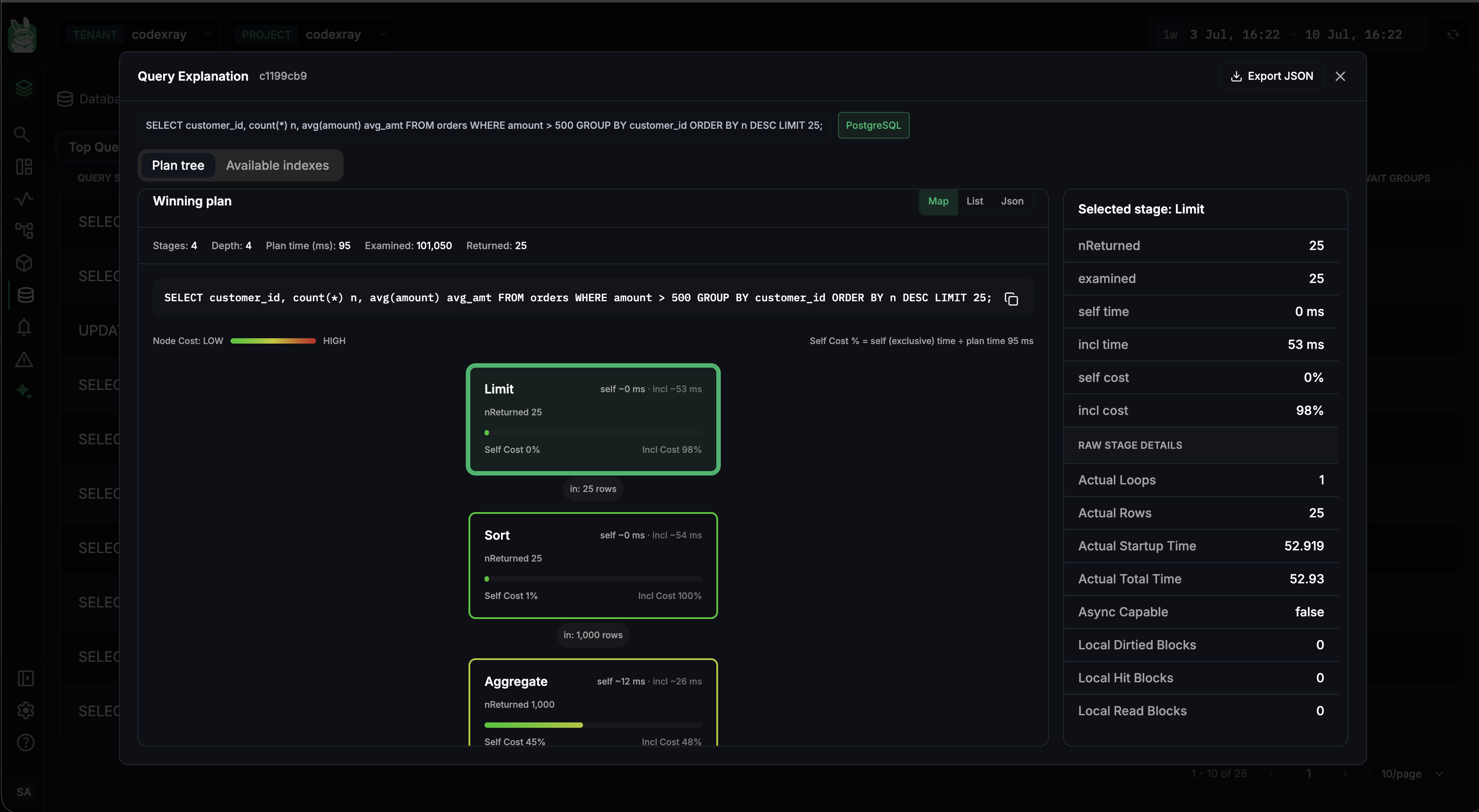
The panel has two tabs — Plan tree and Available indexes — and an Export JSON button in the top-right for taking the raw plan elsewhere (see Exporting the plan below).
Query Explanation is available for queries that have completed at least once. A query that is currently running — one showing up under Currently Running in the Top Queries table — doesn't have a captured plan yet, so the explanation opens only once an execution has finished. If you don't see a plan, the query is still in flight.
Plan tree
The Plan tree tab visualises the query's winning plan as a tree of nodes, so expensive operations stand out immediately. A summary strip surfaces the numbers that matter:
| Stat | Meaning |
|---|---|
| Stages | Number of plan nodes |
| Depth | How deep the plan tree nests |
| Plan time (ms) | Time the planner spent choosing this plan |
| Examined | Rows the engine had to examine |
| Returned | Rows the query actually returned |
The exact query statement sits above the tree with a copy button — one click grabs the SQL to paste into psql, a ticket, or a chat. Switch the plan between Map (the visual tree), List (a flat, sortable stage list), and JSON (the raw plan) to move from a visual overview to raw detail; the JSON view is the quickest way to copy the whole plan without downloading it.
Node cost — reading the colour
Every node is shaded by cost using the Node Cost: LOW → HIGH gradient — green nodes are cheap, red nodes are expensive — so the bottleneck is visible before you read a single number. Each node also shows two percentages:
- Self Cost % — the cost of that node alone (its exclusive time)
- Incl Cost % — the cost of the node plus everything beneath it in the tree
This split is what separates a single expensive operation from an expensive subtree. The panel states the formula it uses right above the tree:
Self Cost % = self (exclusive) time ÷ total query time
So a Sort node at Self Cost 1% / Incl Cost 100% is cheap itself but sits on top of everything; an Aggregate at Self Cost 45% is where the time is actually being spent.
Selected stage — the per-node deep dive
Click any node and the Selected stage panel on the right expands into the single most useful part of the view — a full breakdown of exactly what that stage did:
| Field | What it tells you |
|---|---|
| nReturned | Rows this stage returned |
| examined | Rows this stage had to examine to produce them |
| self time | Time spent in this stage alone |
| incl time | Time including child stages |
| self cost / incl cost | The same split as the tree, for this stage |
| Raw stage details | The planner's raw counters — Actual Loops, Actual Rows, Actual Startup Time, Actual Total Time, Async Capable, Local Hit / Read / Dirtied Blocks, and more |
The examined vs nReturned pair on a single stage is the sharpest signal in the whole panel: a stage examining 100,000 rows to return 25 is scanning far more than it needs to — almost always a missing or unused index.
Look for the node with the highest Incl Cost % first — that subtree is where the query spends its time. Then click it and check its Selected stage panel: a large examined ≫ nReturned gap confirms the query is doing too much work for the rows it returns.
Available indexes
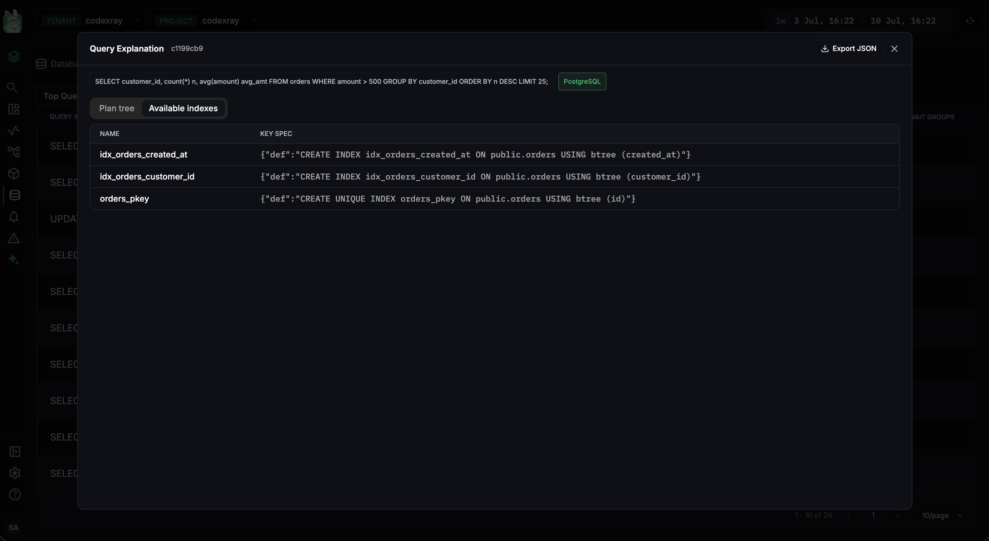
The Available indexes tab lists the indexes relevant to the query, so you can see at a glance whether the plan is using the index you expect or falling back to a sequential scan:
| Column | What it shows |
|---|---|
| NAME | The index name (e.g. idx_orders_customer_id, orders_pkey) |
| KEY SPEC | The full index definition — the CREATE INDEX … USING … statement, including the columns and index method |
It turns "why is this query slow?" into a concrete "this query isn't using index X" in seconds.
Exporting the plan
The Export JSON button hands you the plan as raw JSON — useful for attaching to a ticket, diffing two plans before and after a change, or sharing with a teammate. You can export at two levels:
- The whole query plan — the complete winning plan from the Query Explanation header.
- A single stage's execution — the raw details of the node selected in the Selected stage panel, when you only want to share the one stage that matters.
The JSON view in the Map / List / JSON toggle shows the same content inline if you'd rather read it without leaving the modal.
Plan-tree and available-index inspection is available for PostgreSQL today. MySQL and MSSQL still get the full Top Queries, Metrics, and Active Connections flow above.
Common workflows
"The database is slow — what should I look at first?"
- Open the database from the SQL list and check its Availability and the fleet CPU / Memory KPIs.
- Open Top Queries — sort by Avg Duration or Count. The top 3–5 queries are almost always the cause.
- On PostgreSQL, click the offending query to open its plan tree — a large Examined-vs-Returned gap points straight at a missing index.
- If queries look fine, open Metrics — CPU, Read/Write IOPS, and Outstanding Disk I/O tell a hardware-saturation story that looks different from query-level slowness.
"Connections are piling up — where's the bottleneck?"
- Go straight to Active Connections.
- The By Wait Group chart tells you the shape: CPU-, IO-, or Lock-bound.
- If Lock-bound, the By SQL and By User charts identify the holder.
- By Client reveals which source is driving the connection count.
"Is it the app or the database?"
- Compare the app-side view: Database Insights on the service, scoped to the same time range.
- If app-side query latency ≈ engine-side query latency → the database is the bottleneck (open Metrics).
- If app-side latency ≫ engine-side → look at network, connection pool, or application-layer contention instead.
Next steps
- MongoDB Monitoring — the document-database companion view
- Redis Monitoring — the key-value / cache companion view
- Database Insights — the application-scoped view of the same databases
- CodeXray Database Agent — install and configure the agent that drives these views