MongoDB Monitoring

MongoDB gets its own view in the Databases module, built around the way MongoDB actually works: clusters made of replica-set nodes, operations described by namespace and plan summary, and data organised into databases, collections, and documents. Instead of forcing a relational model onto it, CodeXray gives you a MongoDB-native investigation flow.

Open Databases in the sidebar and switch to the MongoDB tab.

---

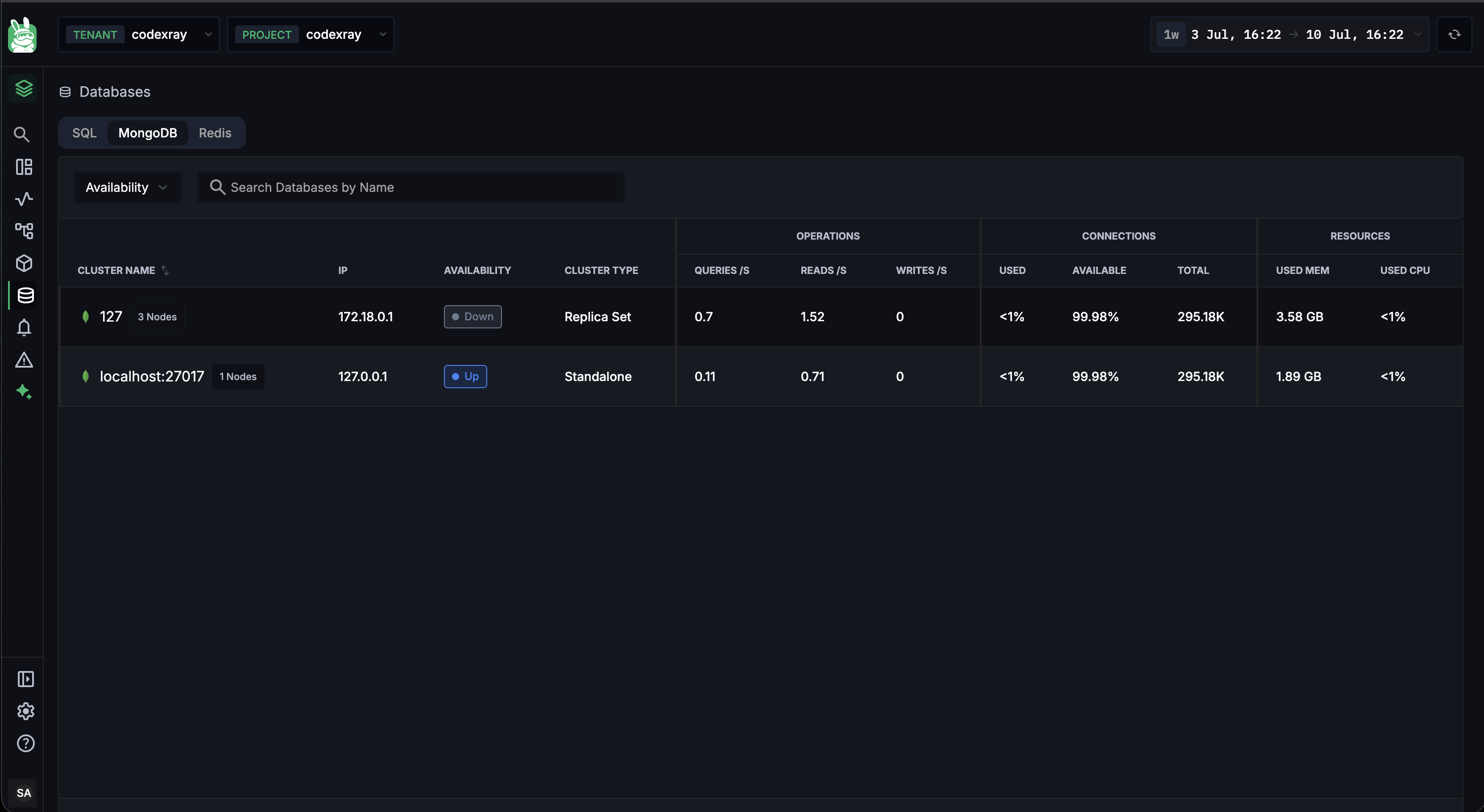
The MongoDB cluster list

The MongoDB tab lists every monitored cluster with signals tuned to document databases:

Column	What it shows
CLUSTER NAME	The cluster name, with a MongoDB icon and a N Nodes badge
IP	Cluster address
AVAILABILITY	Up / Down live status
CLUSTER TYPE	Replica Set / Standalone
OPERATIONS — QUERIES /s	Query operations per second
OPERATIONS — READS /s	Read operations per second
OPERATIONS — WRITES /s	Write operations per second
CONNECTIONS — USED / AVAILABLE / TOTAL	Connection-pool state
RESOURCES — USED MEM	Memory in use (GB)
RESOURCES — USED CPU	CPU utilisation

Use the Search Databases by Name box to find a cluster quickly, then click a row to open the cluster.

---

Cluster detail

Opening a cluster lands you on its overview, with a breadcrumb of Databases › MongoDB › cluster › N Nodes and a set of health charts across the top — Opcounters, Connections, Network In/Out, and Storage — each with its own node selector.

Aligned to the PRIMARY by default

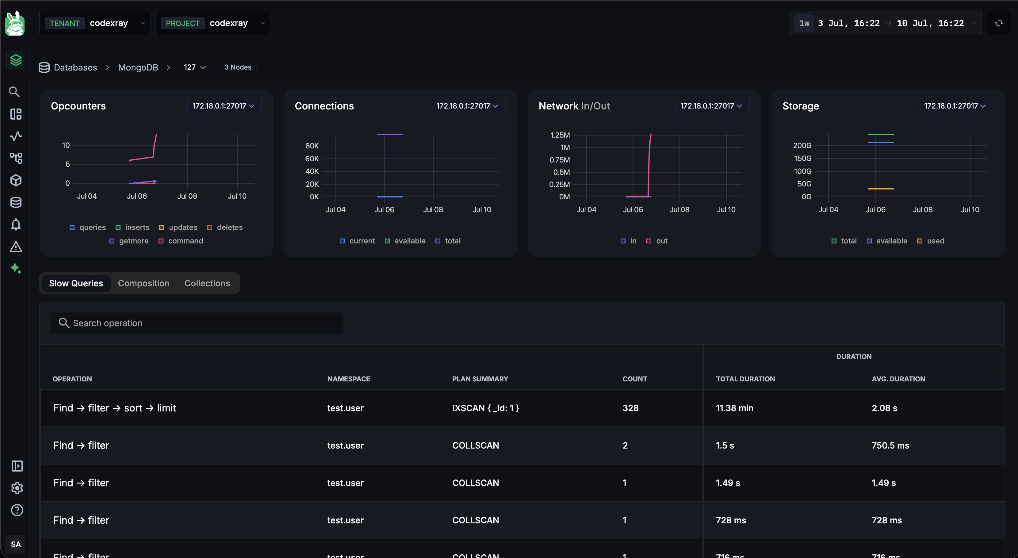
The cluster charts default to the replica set's PRIMARY node — the member taking writes — so what you see first reflects where the load actually lands. Use the node selector to compare a secondary against the primary.

Below the charts, three tabs organise the investigation:

---

Slow Queries

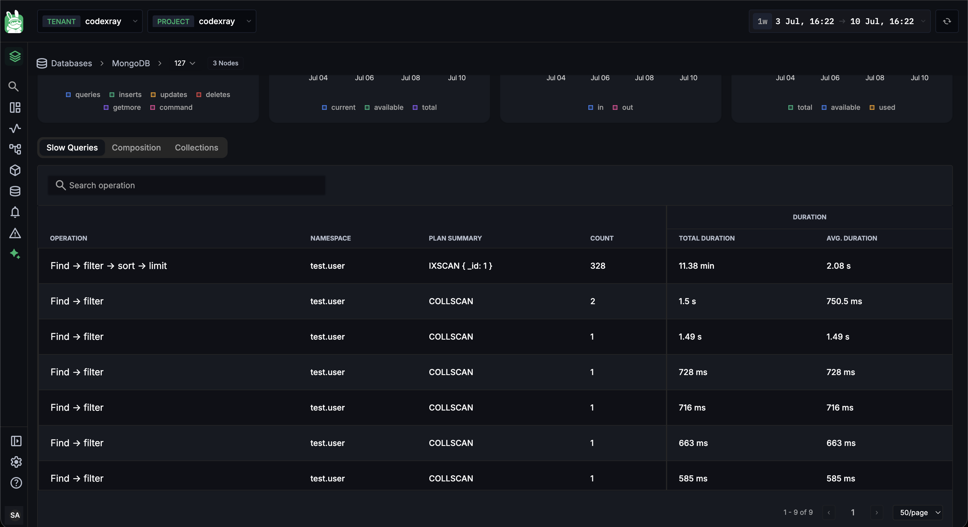
The Slow Queries tab ranks the cluster's slowest operations. Each row describes an operation the MongoDB way:

Column	What it shows
OPERATION	The operation shape (find / aggregate / update / …), with parameters collapsed so variants group together
NAMESPACE	The database.collection the operation ran against
PLAN SUMMARY	How MongoDB executed it — e.g. an index scan (IXSCAN) versus a collection scan (COLLSCAN)
COUNT	How many times the operation ran in the window
DURATION — TOTAL DURATION	Cumulative time spent across all executions
DURATION — AVG. DURATION	Mean execution time

Use the Search operation box to jump to a known operation. PLAN SUMMARY is the fastest tell — a COLLSCAN on a large collection almost always means a missing index.

Click any operation to open its query explanation (below).

---

Query explanation

Click a slow operation and CodeXray opens its execution plan — the same depth of plan inspection MongoDB gives you at the shell, rendered visually.

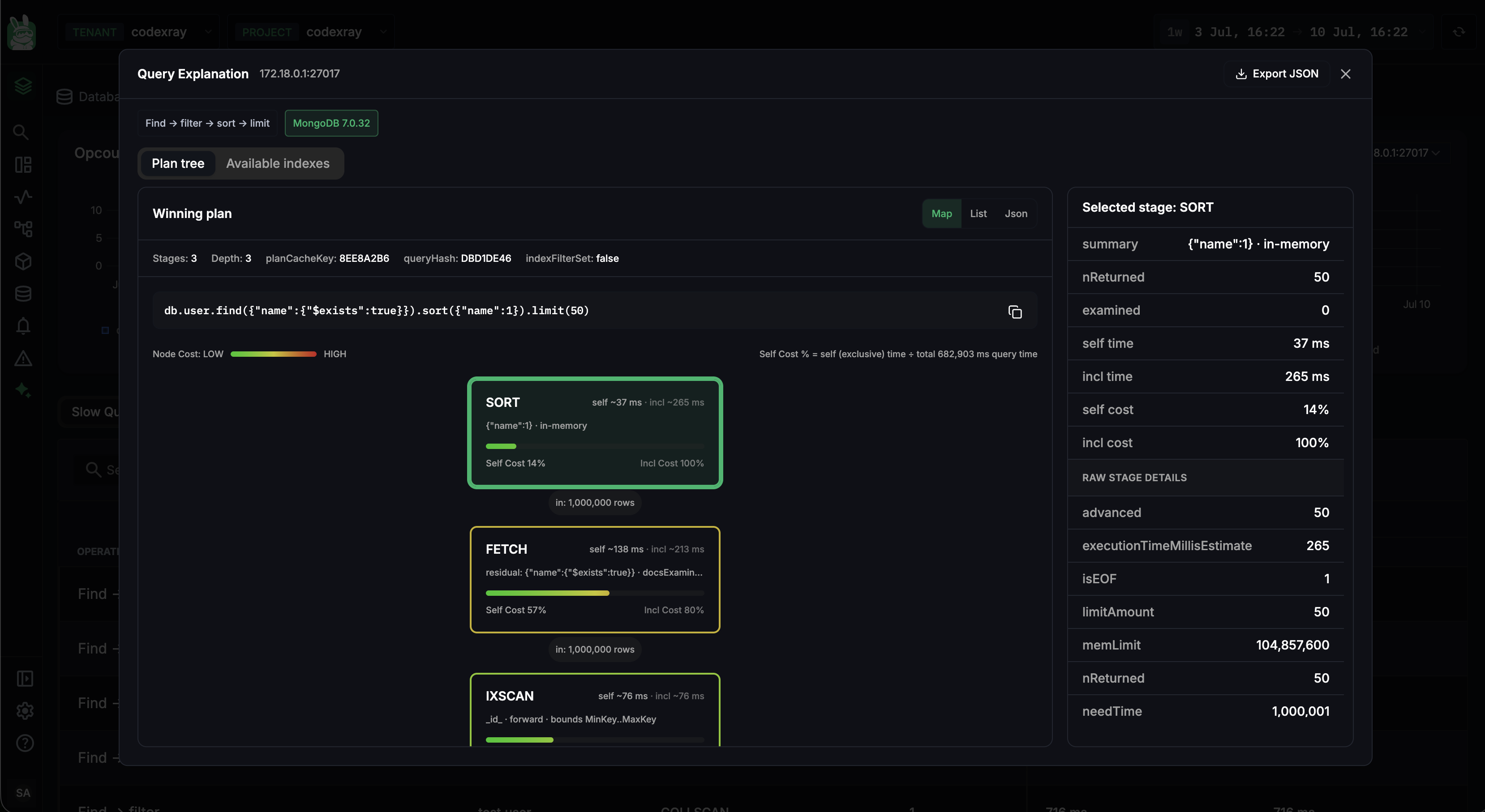
The modal is labelled with the engine and version (MongoDB version), carries an Export JSON button in the top-right, and has two tabs — Plan tree and Available indexes.

Plan tree

The Plan tree tab renders the operation's winning plan as a tree of stages (IXSCAN, FETCH, SORT, COLLSCAN, …). A summary strip surfaces Stages, Depth, and MongoDB's own plan identifiers:

Stat	Meaning
Stages	Number of plan stages
Depth	How deep the plan nests
planCacheKey	MongoDB's cache key for this plan shape
queryHash	Hash identifying the query shape
indexFilterSet	Whether an index filter is forcing the plan

Switch between Map (visual tree), List (a flat table with nReturned, Examined, Time, and Node Cost per stage), and JSON (the raw plan).

Node cost — reading the colour

Each stage is shaded on the Node Cost: LOW → HIGH gradient — cheap stages green, expensive stages red — and shows Self Cost % (that stage alone) and Incl Cost % (the stage plus everything beneath it). The panel prints the formula it uses right above the tree:

Self Cost % = self (exclusive) time ÷ total query time

So a SORT at Self Cost 14% / Incl Cost 100% sits on top of the whole plan, while a FETCH at Self Cost 57% is where the operation actually burns its time.

Selected stage — the per-stage deep dive

Click any stage and the Selected stage panel on the right expands into the most useful part of the view — exactly what that stage did:

Field	What it tells you
summary	The stage's key detail (e.g. {"name":1} · in-memory for a sort)
nReturned	Documents this stage returned
examined	Documents (or keys) it had to examine
self time / incl time	Time in this stage alone, and including child stages
self cost / incl cost	The same split as the tree, for this stage
Raw stage details	MongoDB's raw execution counters — advanced, executionTimeMillisEstimate, isEOF, limitAmount, memLimit, nReturned, needTime, and more

The examined vs nReturned pair is the sharpest signal here: a FETCH or COLLSCAN examining a million documents to return 50 is scanning far more than it needs to.

Available indexes

The Available indexes tab lists the indexes MongoDB could use for this operation — each with its name and key specification — so you can confirm at a glance whether the plan is using the index you expect or scanning the collection.

Exporting the plan

The Export JSON button hands you the plan as raw JSON, at two levels — the whole operation plan from the modal header, or a single stage's execution from the Selected stage panel — handy for attaching to a ticket or diffing a plan before and after adding an index.

From a slow op to a fix

A plan dominated by a COLLSCAN, or a large examined ≫ nReturned gap on any stage, is the signature of a missing or unused index. The Available indexes tab tells you whether the right index exists at all.

---

Composition

The Composition tab shows the cluster as its member nodes, so you can spot an unhealthy or lagging member at a glance. It offers two ways to look:

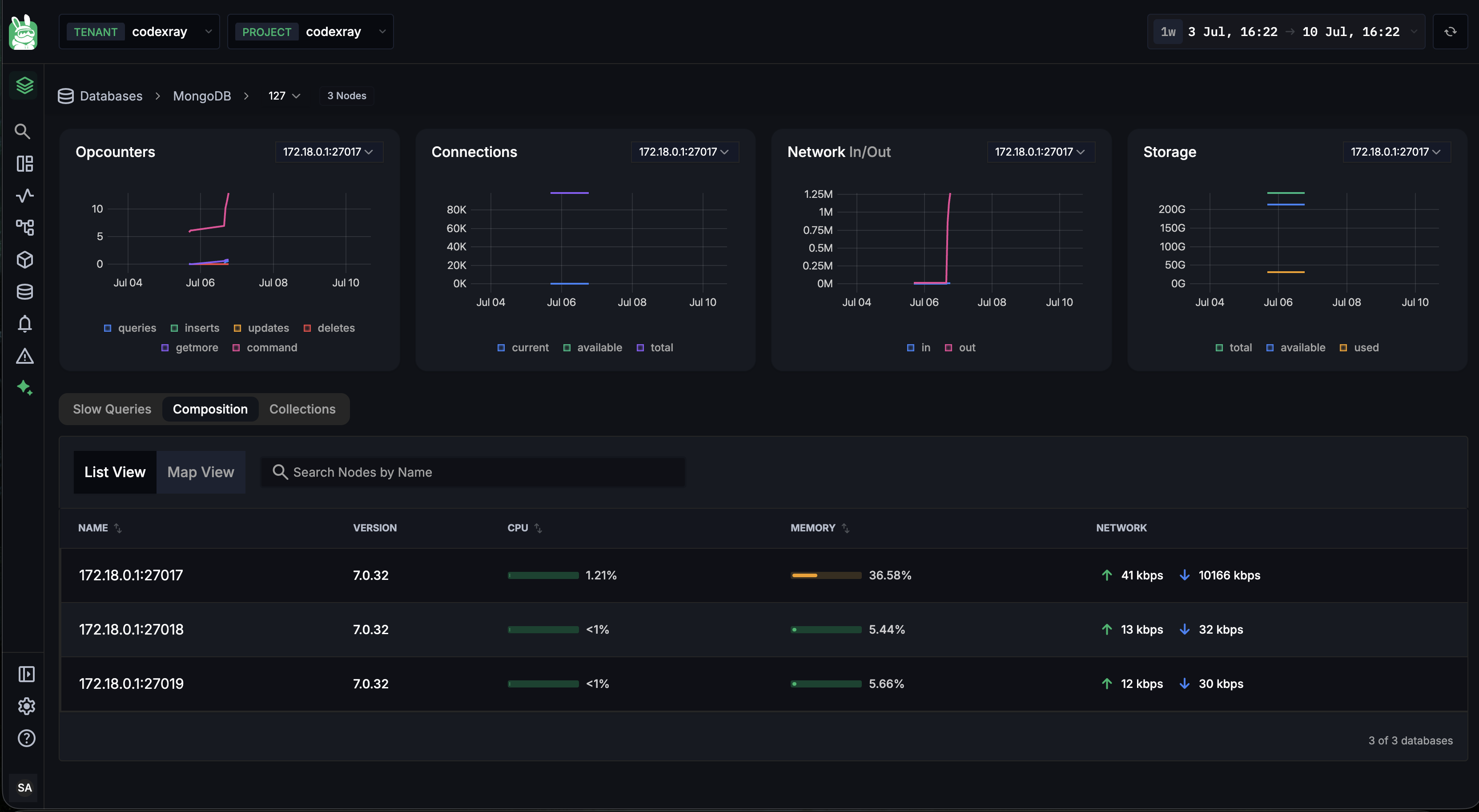
List View — a per-node table:

Column	What it shows
NAME	The node / member name
VERSION	MongoDB version running on the node
CPU	CPU utilisation
MEMORY	Memory in use
NETWORK	Network receive / transmit rate

Map View — the same nodes as a honeycomb layout, grouped by replica-set role (primary / secondary), so the cluster's topology is obvious at a glance and you can see how many members sit in each role.

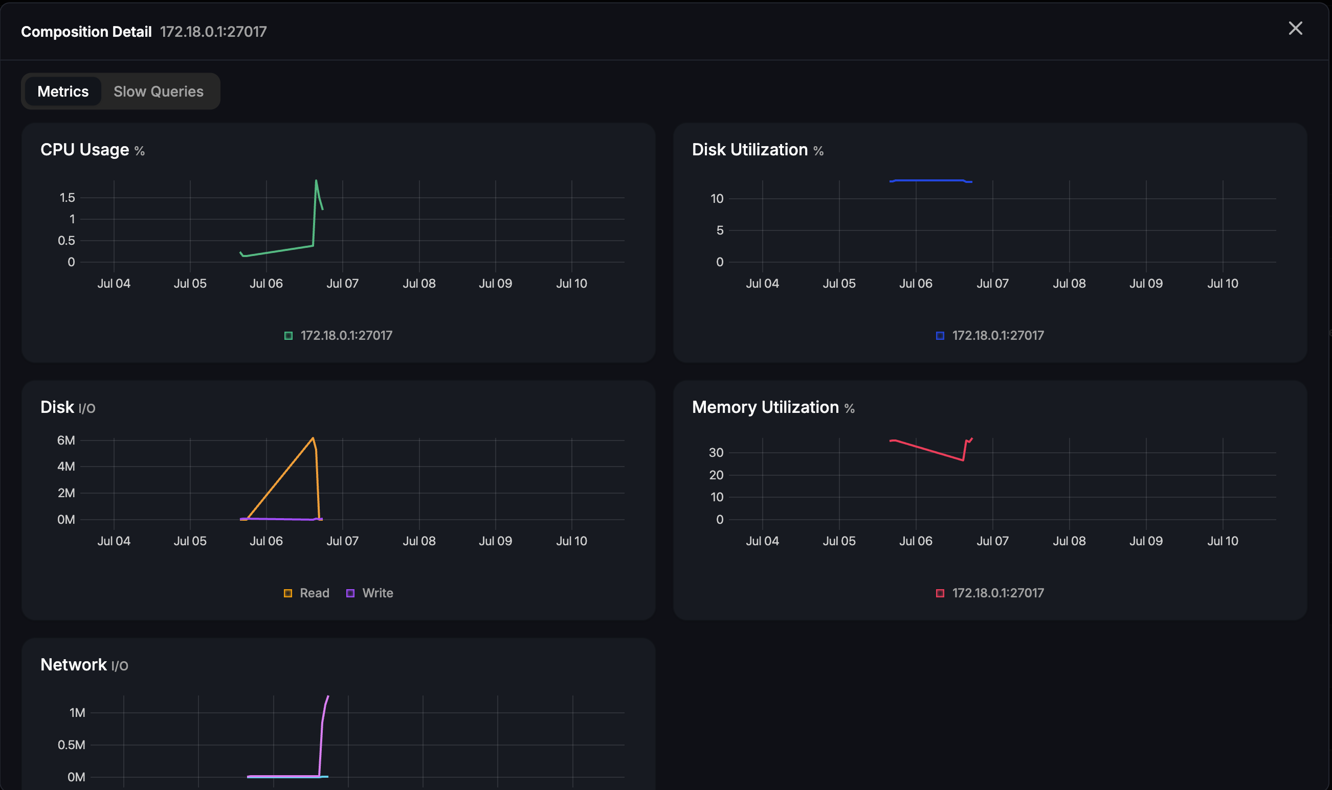
Click any node to open its Composition Detail panel, which has its own Metrics (CPU, disk utilisation, disk I/O, memory, network) and Slow Queries tabs scoped to that single member — useful for confirming whether a problem is cluster-wide or isolated to one node.

---

Collections

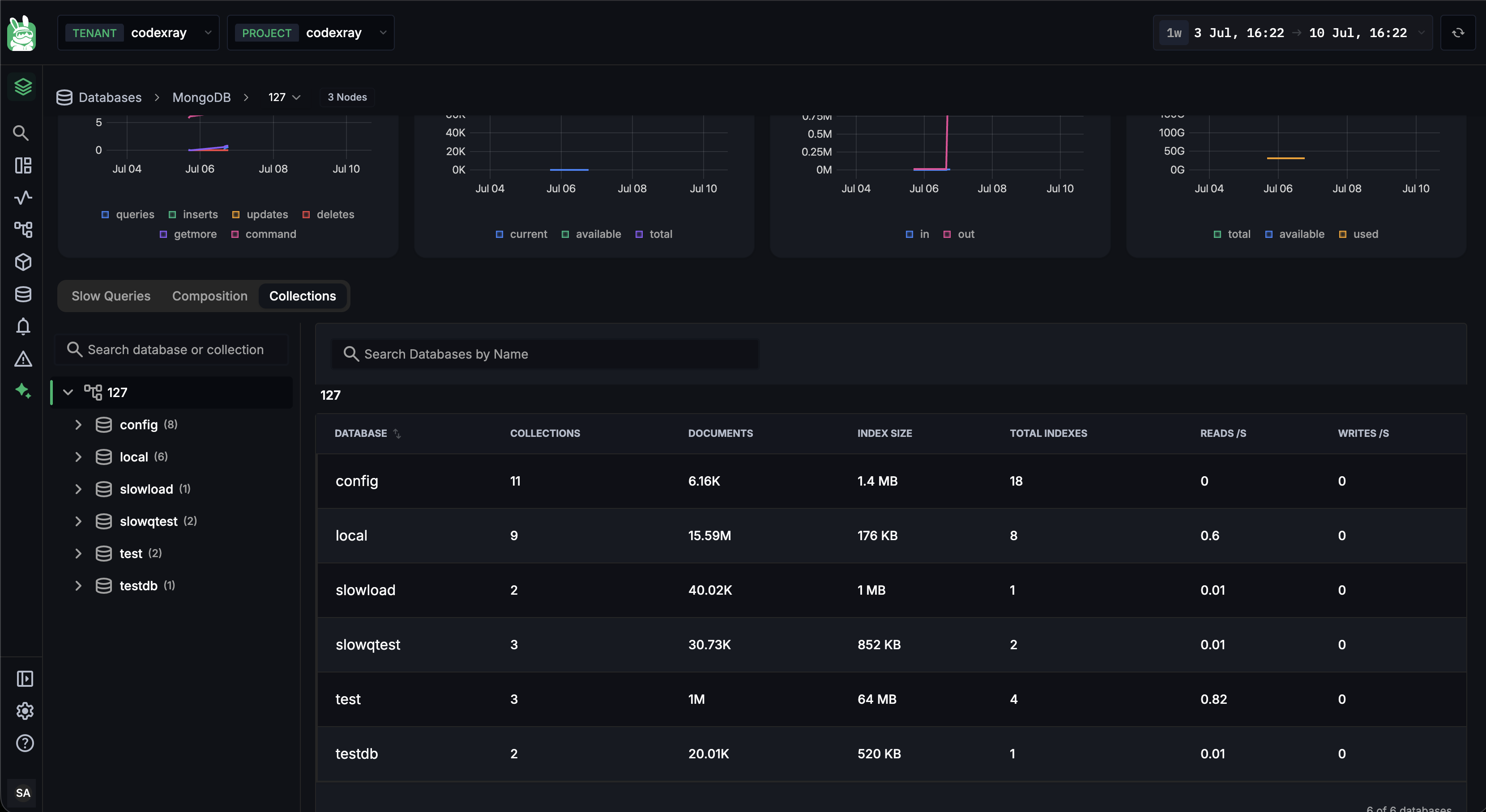
The Collections tab is where you understand the shape of the data. A searchable tree on the left (Search database or collection) lets you drill from the cluster into a database and then into a collection.

Database level:

Column	What it shows
DATABASE	Database name
COLLECTIONS	Number of collections
DOCUMENTS	Total documents
INDEX SIZE	Storage consumed by indexes
TOTAL INDEXES	Number of indexes
READS /s / WRITES /s	Operation rates against the database

Collection level (drill into a database):

Column	What it shows
COLLECTION	Collection name
DOCUMENTS	Documents in the collection
INDEX SIZE	Index storage for the collection
TOTAL INDEXES	Number of indexes on the collection
READS /s / WRITES /s	Operation rates against the collection

Each collection has a View Schema button. Because MongoDB documents are schemaless, CodeXray infers the schema from the data and shows it as a field breakdown:

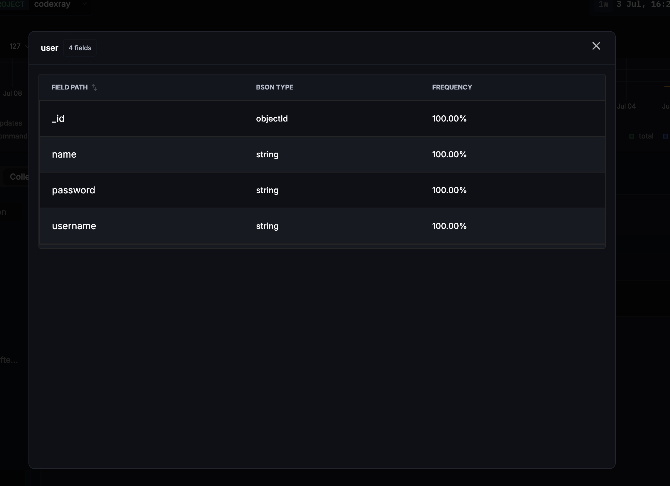
Column	What it shows
FIELD PATH	The document field (including nested paths)
BSON TYPE	The field's BSON type
FREQUENCY	How often the field appears across documents

Why inferred schema matters

A field that appears in only some documents (low FREQUENCY) is a common source of subtle bugs and slow queries — an index on it won't cover the documents that lack it. The schema view makes those inconsistencies visible without scanning the collection yourself.

---

Common workflows

"A MongoDB operation got slow"

1. Open the cluster and go to Slow Queries.
2. Sort by AVG. DURATION or TOTAL DURATION and check the PLAN SUMMARY column — a COLLSCAN is your prime suspect.
3. Click the operation → Query explanation → Plan tree. A big Examined vs nReturned gap confirms an inefficient plan.
4. Open Available indexes to see whether a supporting index exists.

"Is one replica-set member unhealthy?"

1. Open Composition and use Map View to spot an outlier node by colour.
2. Click the node → its Metrics tab to confirm CPU / memory / network pressure.
3. Its Slow Queries tab tells you whether that member is also serving slow operations.

"Which collection is driving load or storage?"

1. Open Collections and sort databases by READS /s, WRITES /s, or INDEX SIZE.
2. Drill into the busiest database, then the busiest collection.
3. Use View Schema to check for inconsistent fields before adding an index.

---

Next steps

• SQL Databases — PostgreSQL, MySQL, and MSSQL monitoring
• Redis Monitoring — the key-value / cache companion view
• Database Insights — the application-scoped view of the same databases
• CodeXray Database Agent — install and configure the agent that drives these views