Distributed Traces — Overview
In a distributed system, a single request may cross many services, databases, and third-party APIs before returning a response. Distributed tracing lets you see that entire path — and CodeXray turns the usual per-trace search into a service-scoped investigation workflow where you start with a visual summary, zoom into the anomalous region, and drill down to individual spans.
See the shape → select the anomaly → understand what's in it → open a single trace for the details.
Where to Find It
Every application in CodeXray has a dedicated Traces tab. Open any service from the Applications list and switch to Traces — everything on the page is scoped to that one service.
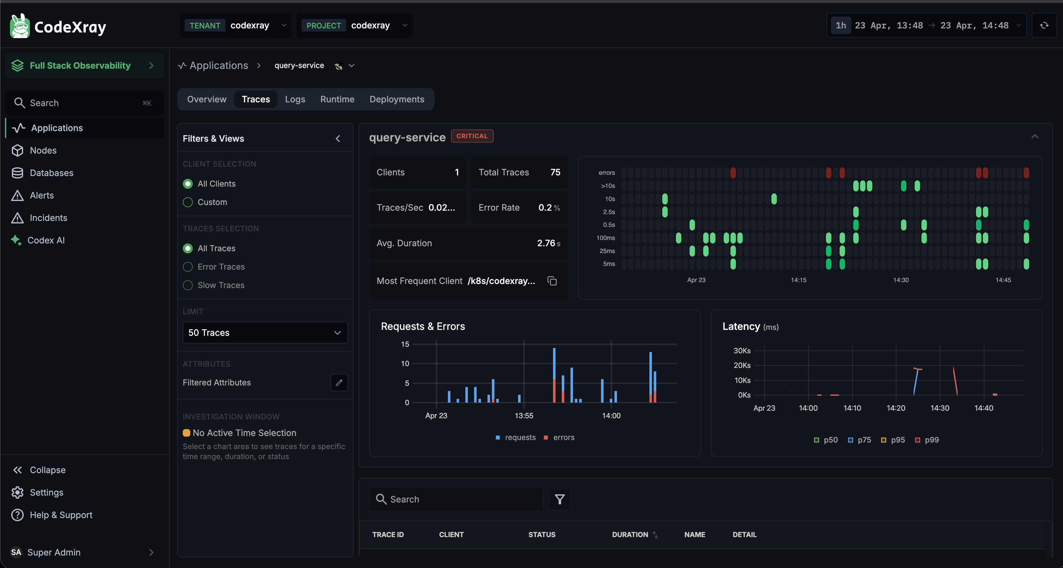
The page is laid out as a guided walkthrough — from a visual summary at the top, through selection-driven drill-down, to individual trace detail and attribute comparison at the bottom.
Anatomy of the Page
1. The Scatter / HeatMap Chart
At the top is a scatter chart plotting every trace in the selected time window. Each dot is one request:
- X-axis — time
- Y-axis — request duration (with a logarithmic scale, from a few milliseconds to 10+ seconds)
- Dot colour — trace status (green = success, red = error)
At a glance you can spot:
- Error spikes — vertical columns of red dots
- Latency anomalies — dots drifting upward away from the normal band
- Volume shifts — density changes across the time axis
Above the chart, a status badge (OK / WARNING / CRITICAL) summarises the service's current health.
2. Summary Stats
The strip below the chart shows the key numbers for the selected time range:
| Stat | What it tells you |
|---|---|
| Clients | How many distinct callers are issuing traces to this service |
| Total Traces | Number of traces in the current window |
| Traces/Sec | Current rate |
| Error Rate | Percentage of traces that failed |
| Avg. Duration | Mean request duration |
| Most Frequent Client | The caller that produced the largest share of traffic |
3. Requests & Errors + Latency Charts
Two charts sit side by side:
- Requests & Errors — a stacked bar chart of request volume (blue) and errors (red) over time. Makes spikes and outages visually obvious.
- Latency (ms) — percentile lines showing p50 / p75 / p95 / p99 over time.
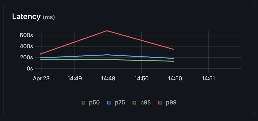
The p99 line is usually where regressions show up first — a spike with p50 still flat means "most users are fine, but the slowest 1% have degraded".
4. Investigation Window — Select a Region to Drill In
This is where CodeXray's tracing gets interesting. Instead of paging through thousands of traces, you click-and-drag a rectangle on the scatter chart to define a time + duration window. Everything below — the Requests & Errors chart, the Latency chart, and the trace list — narrows to exactly that region.
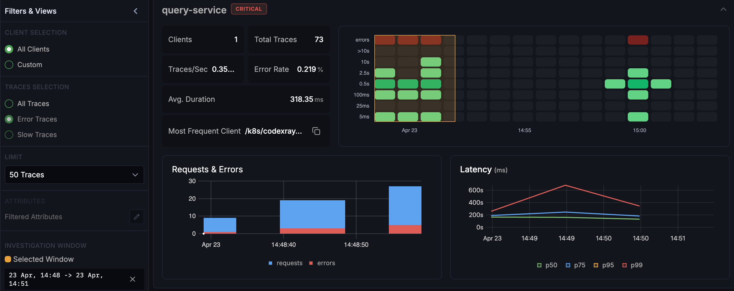
The left filter panel now shows a Selected Window indicator with the exact time range (e.g., "23 Apr, 14:48 → 23 Apr, 14:51") and an × to clear it. The Investigation Window concept makes one thing easy:
I see an anomaly in the chart. Show me only the traces that caused it.
5. The Trace List
Below the charts, the trace table lists individual traces from the current selection (or from the full window if no region is selected). Each row shows:
- TRACE ID — clickable link to the detail view
- CLIENT — the upstream service that made the call
- STATUS — HTTP status code or protocol-specific status badge
- DURATION — total request time
- NAME — operation name
- DETAIL — full URL / endpoint
The left filter panel offers three quick scopes:
- All Traces — everything in the window
- Error Traces — only failures
- Slow Traces — only requests above the latency threshold
Filtering by error traces on a service in trouble instantly narrows the list:
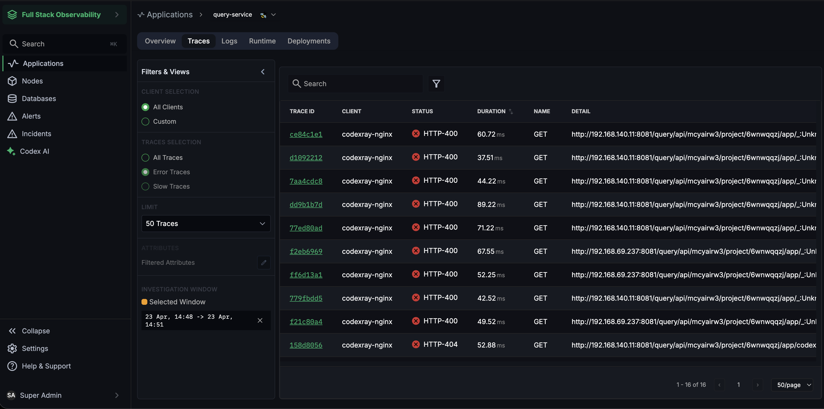
Paired with the selection window, this is the fastest path from "something went wrong" to "here are the 15 traces that match."
6. Trace Detail — Waterfall and Tree Views
Click any trace ID to open the trace detail view — the full span tree for that request.
Waterfall View
The default. Spans are stacked vertically by call depth, aligned against a shared timeline. The longer the bar, the longer the operation. Lower depth = deeper nested calls.
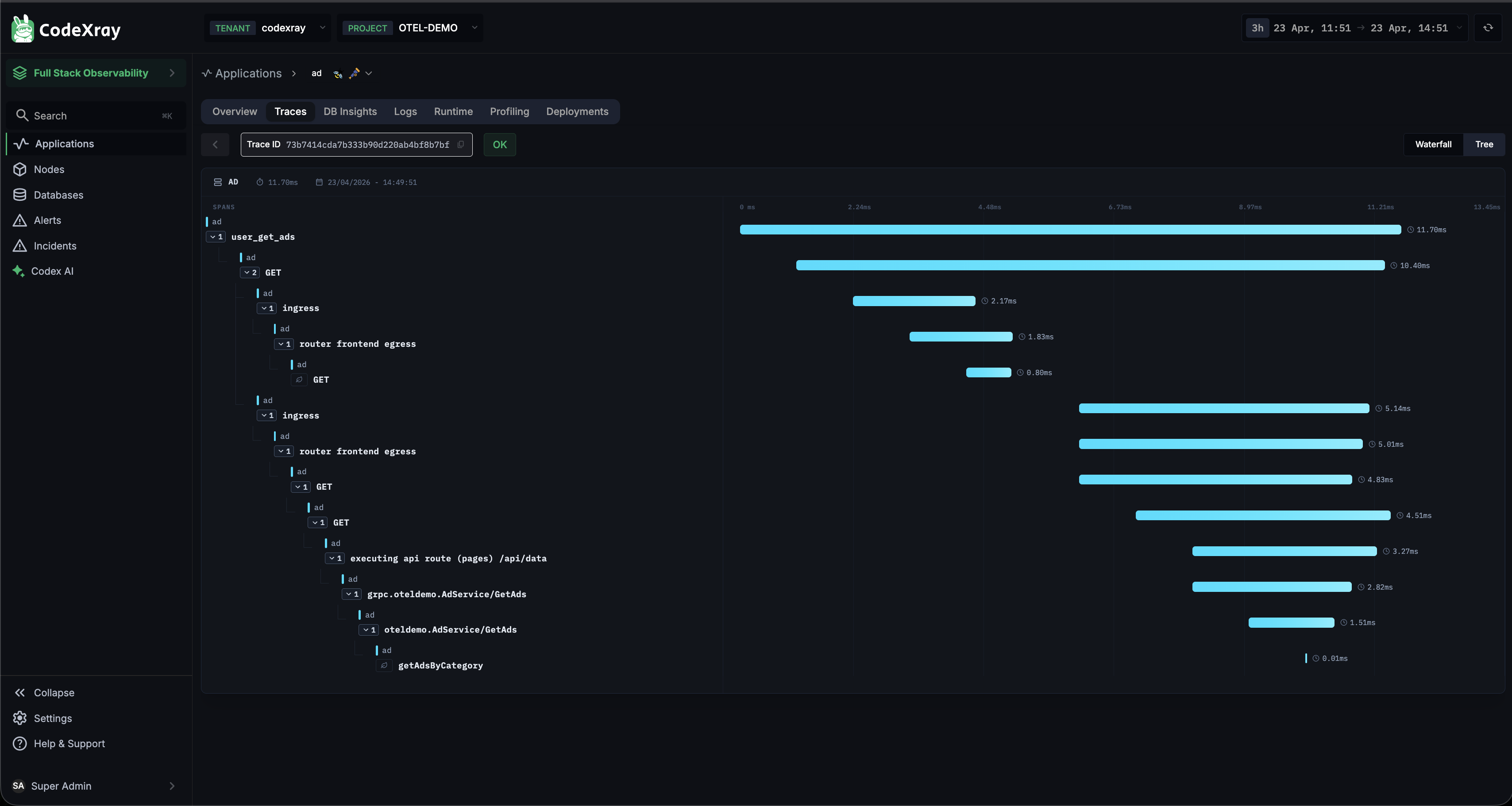
Use Waterfall when you want to see where time is spent. A single long bar at the top with many short children tells a different story from many long bars at the same level.
Tree View
Toggle to Tree in the top-right corner. This renders the trace as a compact horizontal node-link graph — more useful when you have many shallow spans and want to see the request shape rather than per-span durations.
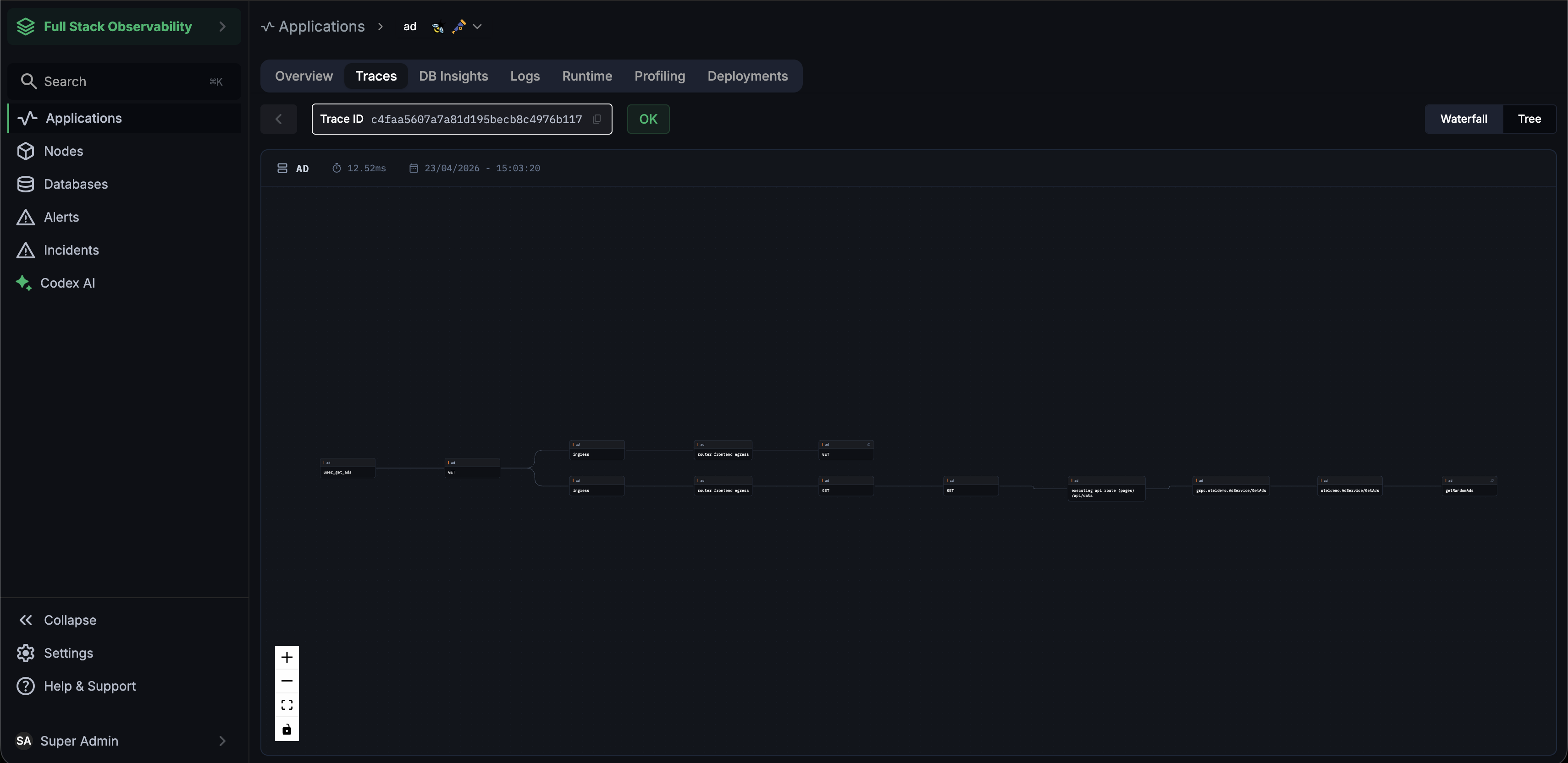
Both views show the same spans — use whichever maps better to the trace you're investigating.
7. Comparative Analysis — Latency Explorer and Compare Attributes
Once you've used the chart + selection workflow to narrow down to an anomaly, CodeXray offers a deeper investigation mode: Comparative Analysis. Toggle it on from the filter panel and the page switches from "here are the traces" to "here's how these traces differ from the rest."
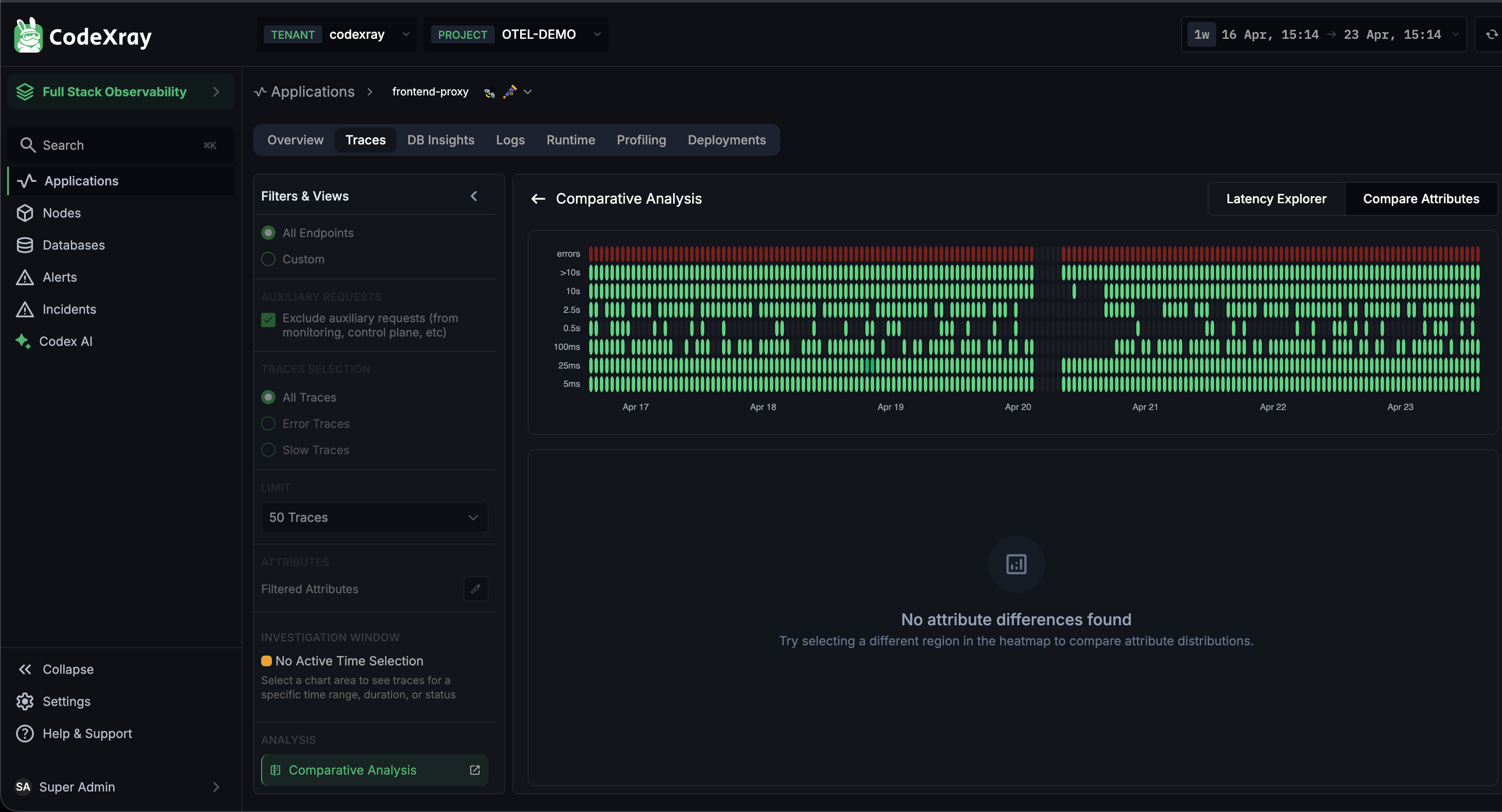
Two sub-tabs sit at the top right:
Latency Explorer
A high-resolution heatmap of request distribution across a long time window — every request plotted by duration and timestamp. Dense green bands show the "normal" latency profile; outliers stand out above them.
Drag to select any region on this heatmap and the rest of the page — including the Compare Attributes tab — scopes to just those traces. Use it when:
- You want to characterise latency over a long window (days, not minutes) and spot recurring slow patterns
- You want to isolate a specific latency band ("requests taking 1–3 seconds") and see what they have in common
A checkbox in the filter panel — Exclude auxiliary requests (from monitoring, control plane, etc.) — removes low-signal traffic like health checks, readiness probes, and internal heartbeats. On by default for clearer analysis; untick it if you specifically need to include them.
Compare Attributes
Once a region is selected in the Latency Explorer, the Compare Attributes tab answers:
What makes these requests different from all the others?
It compares trace attributes between the selection and the baseline and surfaces statistically meaningful differences — for example, "93% of selected requests have feature_flag=new_checkout enabled, vs 12% baseline" or "all selected requests originate from the mumbai region."
Works with any attribute — OTel semantic conventions (http.method, db.system, etc.), resource attributes (service.version, deployment.environment), or custom attributes your app sets. No configuration required; CodeXray discovers and compares attributes automatically.
This is the feature that closes the "why is it slow?" question — especially for issues that only affect a specific customer, browser, version, or region.
How Traces Reach CodeXray
CodeXray ingests spans from two complementary sources:
1. OpenTelemetry SDKs
The rich path. Applications instrumented with OpenTelemetry emit OTLP traces directly to the CodeXray collector — with full span trees, custom attributes, and trace context propagated across every hop. Dedicated setup pages for the most common languages:
Any language with OpenTelemetry SDK support (Node.js, Ruby, PHP, Rust, .NET, C++) works too — just point the OTLP exporter at the CodeXray collector.
2. eBPF-based Tracing
The zero-code path. The CodeXray Node Agent captures outbound requests at the kernel via eBPF and converts them into OTel spans automatically. Auto-instrumented protocols: HTTP, gRPC, PostgreSQL, MySQL, MongoDB, Redis, Memcached, RabbitMQ, Kafka.
Both sources land as OTel spans in the same store. You can mix them freely — eBPF traces for services you haven't instrumented yet, SDK traces for the ones you have.
Supported Languages
CodeXray accepts OTLP from any OpenTelemetry-compliant language. Dedicated setup guides are available for the three most common:
| Language | Instrumentation style | Dedicated guide |
|---|---|---|
| Java | Automatic via opentelemetry-javaagent.jar — zero code changes | OpenTelemetry for Java |
| Python | Automatic via opentelemetry-instrument | OpenTelemetry for Python |
| Go | Manual SDK integration (no auto-instrumentation available in OTel Go) | OpenTelemetry for Go |
| Node.js | Automatic via --require @opentelemetry/auto-instrumentations-node/register | — (use standard OTel docs) |
| .NET | Via CodeXray .NET Agent (legacy + modern) or OpenTelemetry.AutoInstrumentation | .NET Agent |
| Ruby / PHP / Rust | Via standard OpenTelemetry SDKs and OTLP exporters | — (use standard OTel docs) |
All roads lead to the same OTLP collector endpoint. Pick whichever matches your language and you're done.
Pairs Well With
Tracing is most powerful when correlated with other signals:
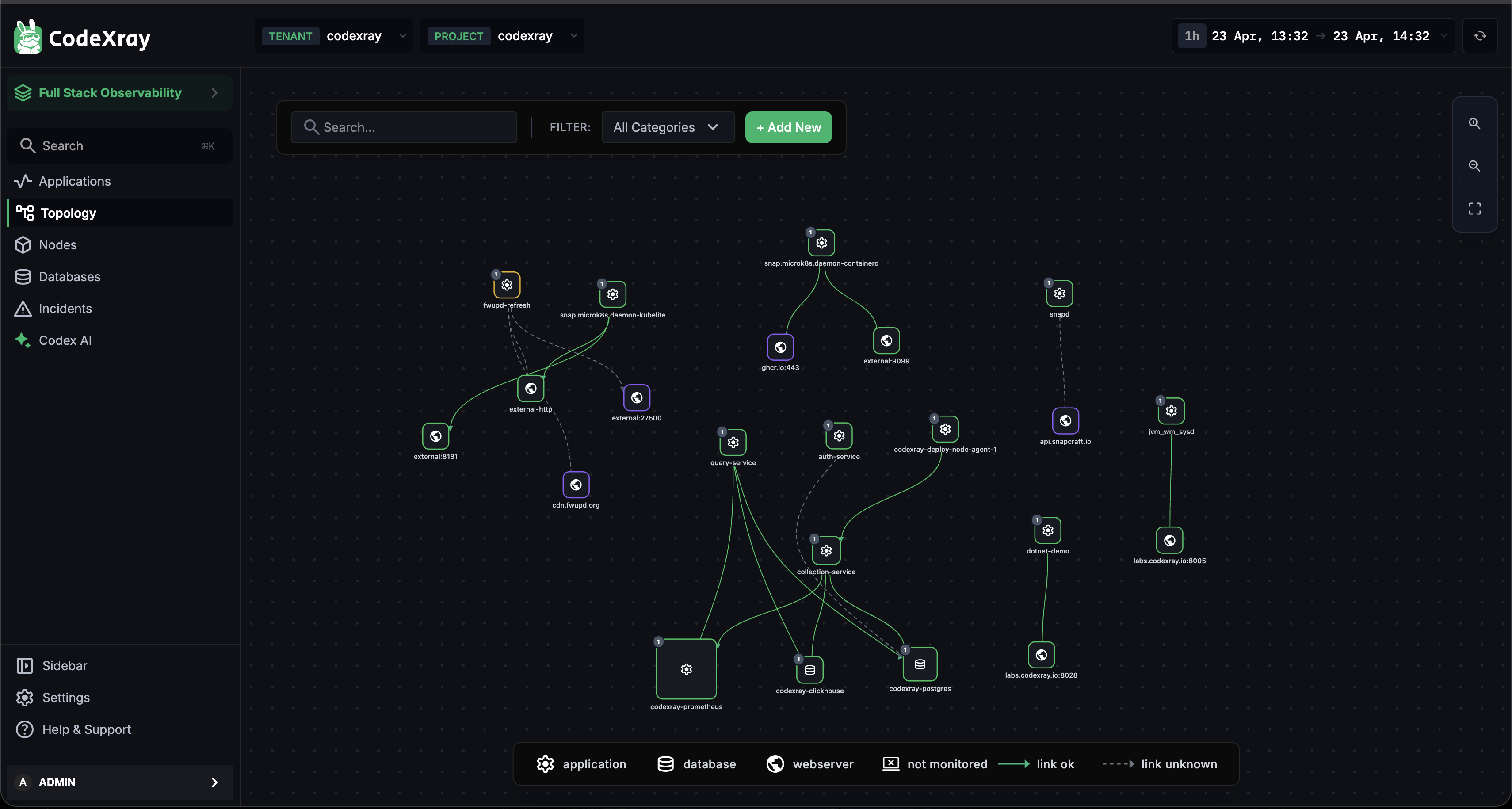
- Service Map / Topology — the Topology view visualises every service discovered from traces (and from eBPF)
- Logs — see the Log Monitoring section to pivot from a log line to its trace
- DB Insights — every trace's database calls surface in the Database Insights tab
Next Steps
- eBPF-based Tracing — how the Node Agent captures traces with zero code changes
- OpenTelemetry for Java · for Python · for Go — language-specific setup guides
- Architecture — how tracing fits into the CodeXray platform