Continuous Profiling — Overview
Continuous Profiling lets you identify and analyze unexpected spikes in CPU usage down to the precise line of code.
Unlike ad-hoc profiling that you run when something's already broken, CodeXray's profiler is always on. So when an incident hits, you can look back and compare "how was my code behaving an hour ago vs. now?" without needing to reproduce the problem.
CPU dashboards tell you a node is hot. Traces tell you which request was slow. Only profiles tell you which line of code burned the CPU. For most performance investigations, the profiler answers the question faster than anything else.
Where to Find It
Every application has a dedicated Profiling tab alongside Overview, Traces, Logs, Runtime, and Deployments.
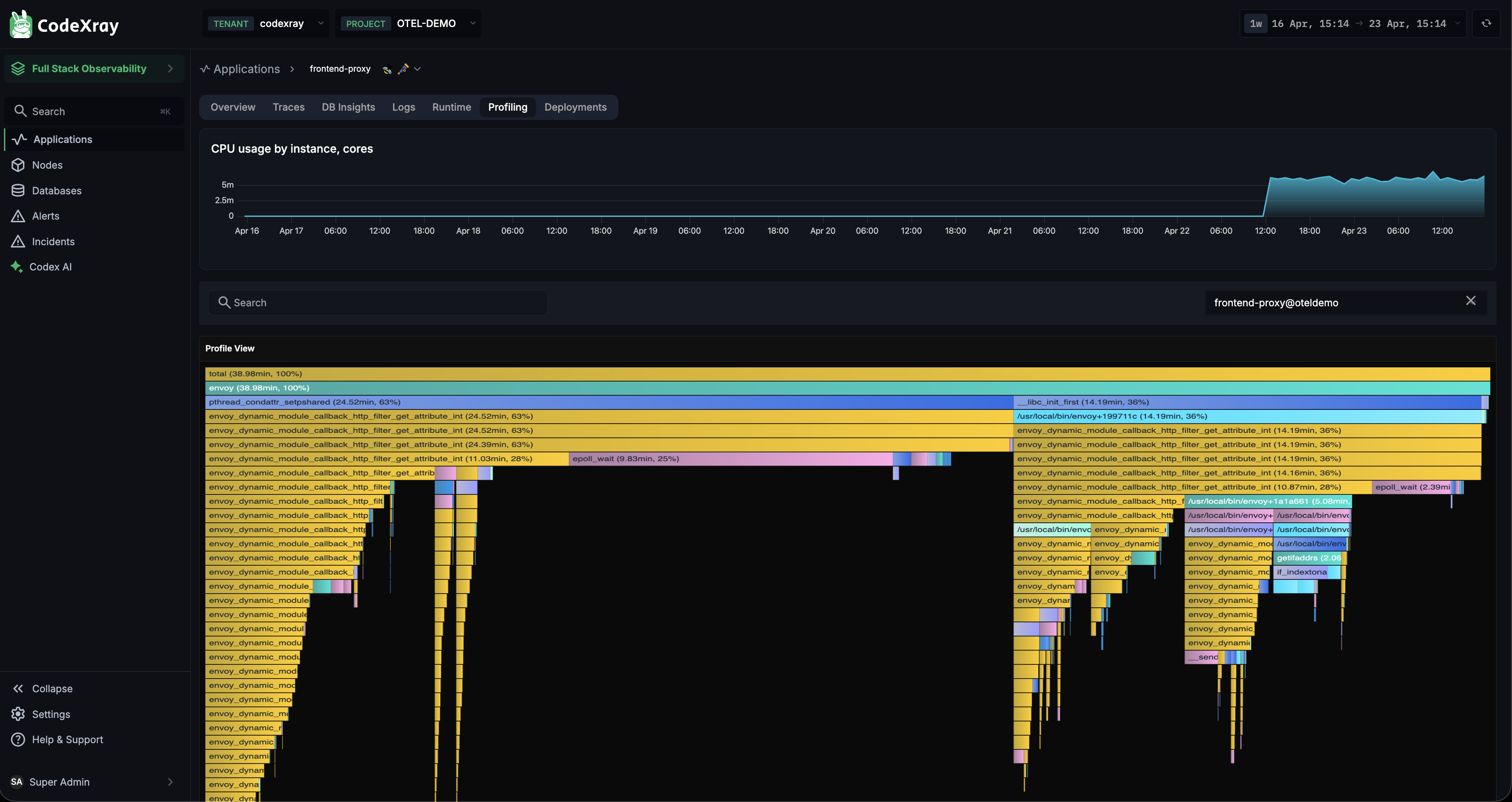
The page has two regions:
- CPU usage by instance, cores — a time-series chart at the top showing live CPU consumption over the selected window. Pick any range here to scope the FlameGraph below.
- FlameGraph — the visualisation of the aggregated profile for that window.
Reading a FlameGraph
The FlameGraph organises the code hierarchy by CPU time consumption:
- Each frame is a function
- Width = CPU time consumed — wider means hotter
- Frames underneath represent nested function calls (call stack grows downward)
- Colour is determined by the package — functions from the same package share the same colour
You read a FlameGraph from top to bottom:
- The wide frames near the top are the entry points
- Follow them down the stack to find the deepest hot frame — that's usually where the CPU actually went
Use the Search box above the FlameGraph to filter by function name — handy when you know what you're looking for.
Zoom Mode vs Comparison Mode
Select any region on the time-series chart above the FlameGraph and you get two mode options:
Zoom mode
Scope the FlameGraph to just that time sub-range. Useful when a spike is visually isolated and you want to see exactly what was running.
Comparison mode
Split the selected range against the surrounding baseline and render two FlameGraphs side by side — left is the baseline, right is the selected (anomalous) window. The right-hand graph uses colour to show what changed:
- Red frames — functions consuming more CPU vs. baseline (the ones that got worse)
- Green frames — functions consuming less CPU (improvements or cooler paths)
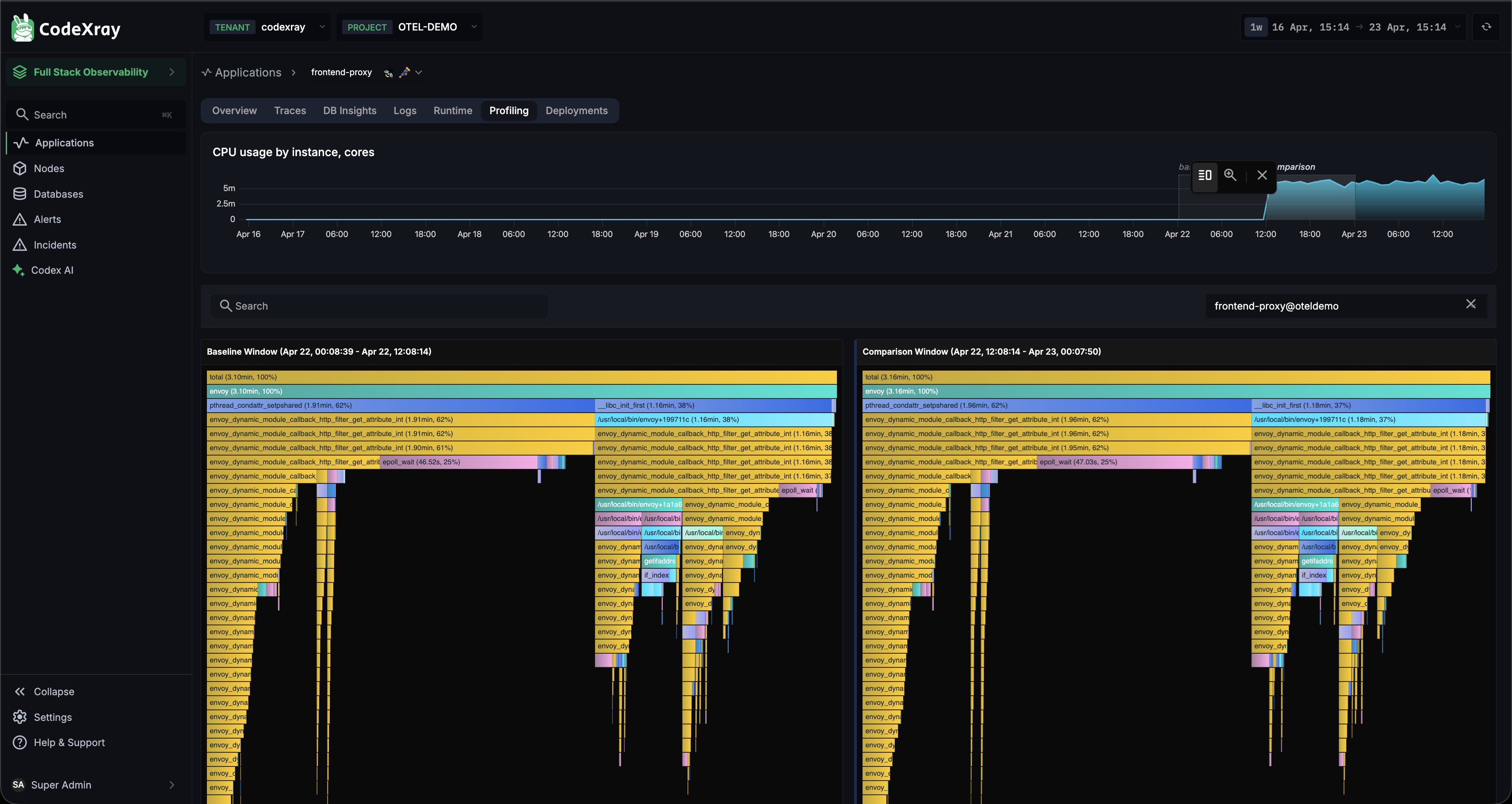
This is how you answer "what changed?" — especially useful right after a deploy, a traffic shift, or an incident.
How Profiles Reach CodeXray
Profiles are captured by the CodeXray Node Agent, which runs an eBPF CPU profiler that samples stack traces from the kernel for every process on the host — no code changes, no SDK, no application-side setup.
Supported languages: Go, Python, Java (JVM), and native code (C, C++, Rust, and other compiled binaries).
Profile types: CPU. See eBPF-based Profiling for the full story.
Java specifics
Java profiling runs over the eBPF path, but the Node Agent does some JVM-specific work (attaches to the JVM over the attach socket and dumps a perfmap) so Java method names resolve correctly in the FlameGraph. See Java Profiling for the JVM flag you need to set.
CPU / Memory Shortcut Tabs
In addition to the Profiling tab, the CPU and Memory tabs on the application page link directly to the CPU and memory FlameGraphs respectively. A one-click path from "this chart is spiky" to "show me the code".
Getting Started
- Install the Node Agent — it starts profiling every process on every node it runs on. Within a few minutes, any service will show a FlameGraph in its Profiling tab.
- For Java apps: add
-XX:+PreserveFramePointerto your JVM options — see Java Profiling.
Next Steps
- eBPF-based Profiling — how the always-on, zero-code CPU profiler works
- Java Profiling — the JVM flag and setup details
- CodeXray Node Agent — the agent that runs the eBPF profiler